Updating Triangulations.

1. Introduction.

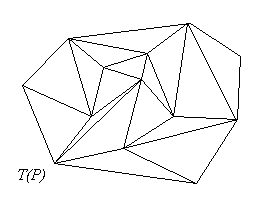
Figure 1.0.A triangulation of a set of points.

Although the problem of constructing a triangulation given a set of points or a simple polygon has been paid considerable attention, at times, in various contexts, it is also necessary to update existing triangulations by inserting or deleting some vertices or edges. Some strategies to do that are considered in this page.

2. Nodes.

If $p$ is located in the interior of the convex hull of $P$ it must lie inside some triangle $t$ of $T(P)$. In which case, it is, possible to connect $p$ to the vertices of $t$ obtaining a valid triangulation (see Figure 2.0 A, point $p$).

Alternativelly, some inserted point $p\text{'}$ may happen to overlay some edge. For this particular problem such a degeneracy can be trivially handled by splitting the edge at the inserted vertex and adding another new edge into every triangle the original edge was a member of (see Figure 2.0 A, point $p\text{'}$).

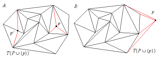
Figure 2.0. Inserting a vertex into a triangulation.

Note that we can easily create the list of the vertices on the boundary of the hole by traversing the triangles of the triangulation (Assuming, of course that an efficient data-structure which chains all triangles is used).

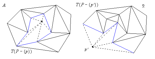
Figure 2.1 Deleting a vertex from a triangulation.

3. Edges.

The following subsections discuss different cases of edge insertion/deletion.

3.1 Inserting an edge into a triangulation.

• Connect with an edge two nodes $p$_i and $p$_j in the case when both belong to the set $P$ (Insert an "open" edge).
• Connect with an edge two nodes $p$_i and $p$_j in the case when both don't belong to the set $P$ (Insert a "closed" edge).

3.1.1 Inserting an open edge.

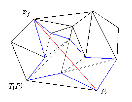
Figure 3.1. Inserting an open edge into a triangulation.

3.1.2 Inserting a closed edge.

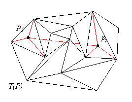
Figure 3.2. Inserting a closed edge into a triangulation.

3.2 Deleting an edge from a triangulation.

• Delete an edge along with its end-points: $p$_i and $p$_j (delete a "closed" edge).
• Delete (if possible) the edge connecting some nodes $p$_i ,$p$_j but leave the end-points in the set $P$ (delete an "open" edge).

3.2.1 Deleting a closed edge.

Although this computation takes linear time, we may do somewhat better by avoiding triangulation of two star-shaped holes (together resulting in application of three-coins algorithm up to six times) and directly construct some edge-visible holes requiring only four application of the triangulation algorithm.

Thus we start by extending the edge we want to delete, find its intersections with some other edges on the boundary of the formed hole. Further, we insert these Steiner points into the set, triangulate the formed edge-visible polygons, remove the Steiner points and obtain other edge visible polygons which can be trivially triangulated (see Figure 3.3).

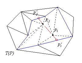
Figure 3.3. Deleting a closed edge from a triangulation.

3.2.2 Deleting an open edge.

Clearly, this may not always be possible (see Figure 3.4 A). Edge $e$ cannot be deleted from the triangulation $T(P)$.

To delete an open edge we must find two other points from the set $P$, $p\text{'}$_i and $p\text{'}$_j whose connecting line (a stabbing line) intersects the edge we want to delete. Insertion of an edge $p\text{'}$_i,p_j necessarily deletes the edge $p$_i,p_j solving the open edge deletion problem.

One straightforward way of finding a stabbing line is by checking all pairs of points from the set $P$ to verify if any intersects the edge we want to delete. To speedup this quadratic computation we can precompute the required information ( whether the edges intersect ) in a square array, use it to fetch stabbing edges in unit time and make sure we adjust the array according to the triangulation updates.

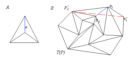
Figure 3.4. Deleting an open edge from a triangulation.

Although this algorithm fails in finding a correct convex hull of a general simple polygon, it does work for an important class of polygons, notably those which are weakly externally visible. A polygon is called weakly externally visible if any point on its border is directly visible from some point located at infinity.

This algorithm can be described as follows:

for n points of a polygon: k,k+1,...,k+n-1, starting with k=0 which
is assumed to be convex.
do
 if (k,k+1,k+2) are counterclockwise triple and k+2=n then stop
 else
  if (k,k+1,k+2) are counterclockwise then move one point forward
  else
  begin
    delete k+1, add diagonal (k,k+2)
    if k=n then move one point forward
    else move one point backward
  end
end

The algorithm proceeds by finding and closing with a lid each encountered pocket (see Figure 4.1).

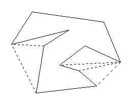
Figure 4.1 Applying the three-coins algorithm.

Note that in the process of finding a lid each of the pockets has been externally triangulated.

The suggested algorithm, however, assumes that no three vertices in the polygon are collinear. In the presence of such degeneracies a modified version of the three-coins algorithm should be used.

for n points of a polygon: v,k,k+1,...,k+n-2,u such that
uv is the visibility edge, and a stack S so that s is stack's top.
push v
push k
assign x=k+1
do
 if x=v stop
 if (s-1,s,x) are counterclockwise or 0 degree turn triple then
 begin
   push x
   move x one point forward
 end else begin
   if (s-1,x,x+1) is a 180 degrees turn then
   then add diagonal (s,x+1), move x one point forward
   else add diagonal (s-1,x), pop stack
 end
 if s=v then
 begin
   push x
   move x one point forward
 end
end

Since the three-coins algorithm was capable of externally triangulating the pockets (which are edge visible polygons with respect to the lid) we can internally triangulate any edge-visible polygon using the above algorithm in linear time (see Figure 4.2).

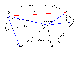
Figure 4.2 Triangulating an edge-visible polygon.

If we are given a point in the kernel such polygons can be triangulated using a variation of the three-coins algorithms. Notably we want to first insert an edge originating in some vertex and passing through the kernel. This edge may intersect some other edge on the other side at which place we will introduce a Steiner point. The resulting two edge-visible polygons can be efficiently triangulated (the newly inserted visibility edge passes through the kernel and hence all points in both halves are visible).

Afterwards, we remove the Steiner point and invoke the three-coins triangulation once again to fill the formed hole which was edge visible since the removed point was originally placed onto an edge (see Figure 4.3).

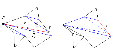
Figure 4.3 Triangulating a star-shaped polygon.

5. References.

• [1] H.A. ElGindy, G.T. Toussaint, "Efficient algorithms for inserting and deleting edges from triangulations." Proc. International Conference on Foundations of Data Organisation, Kyoto University, 1985.
• [2] G.T. Toussaint, D. Avis, "On a convex hull algorithm for polygons and its application to triangulation problems," Pattern Recognition, Vol. 15, 1982, pp. 32-29.
• [3] A.A. Schone, J. van-Leeuwen, "Triangulating a star-shaped polygon," Technical Report RUV-CS-80-3, University of Utrecht, April 1980.
• [4] R.L. Graham, "An efficient algorithm for determining the convex hull of a finite planar set," Inform. Process. Lett. 1, pp. 132-133, 1972.
• [5] J. Sklansky, "Measuring concavity on a rectangular mosaic," IEEE Transactions on Computing. C-21, pp. 1355-1364, 1972.
• [6] P. Bose, G.T. Toussaint, "Growing a tree from its branches," Journal of Algorithms. 19, pp. 86-103, 1995.